Wellcome! This page is about theory representation and scientific inference with first order logic, including the written documentation for Theory Toolbox 2.

Below you can find a written guide to logic programming, theory representation and inference with Theory Toolbox 2. Rohner and Kjellerstrand (2021) contains a theoretical discussion of theory representation in psychology. This webpage is a living document; if you find and problems or have suggestions for improvement please post an issue.

1. Overview

• Section 2 explains how to run Theory Toolbox 2.
• Section 3 gives a quick introduction to logic programming.
• Section 4 explains some basic principles for designing scientific theories.
• Section 5 discusses the advantages of logic programming with respect to theory representation.
• Section 6 shows how to use Theory Toolbox 2 for inference, explanation, theory evaluation and theory construction.

2. Running Theory Toolbox 2

To run Theory Toolbox 2 you have two options: (1) Go to the Playground, or (2) Install Theory Toolbox 2 and SWI Prolog (Wielemaker et al., 2011) on your local machine by following the steps in sections 2.1 and 2.2 below. So if you opt for the playground you do not have to install anything; the playground uses SWISH in your browser (Wielemaker et al., 2015).

2.1. Local Installation

It is possible to run SWI-Prolog from Terminal on Mac or the command line in Windows. However, using Visual Studio Code is very handy: It has built in GitHub support and you can define user snippets for different logical symbols. To setup everything to work with Visual Studio Code follow these steps:

1. Download and install SWI Prolog.
2. Download and install Visual Studio Code.
3. Install the VSC Prolog extension
   • Start Visual Studio Code and click the extensions symbol in the side bar on the far left (the symbol with four squares).
   • Search for the VSC Prolog extension and install it.
4. Download the Theory Toolbox 2 repository
   • Using your web browser navigate to the theory-toolbox-2 repository.
   • Click the green Code button and chose Download ZIP
   • Unpack the folder somewhere on you hard drive
   • In Visual Studio Code, click the File menu, choose Open Folder, and open the theory-toolbox-2 folder.
5. Load an example
   • In the folder structure to the left double click an example, e.g. substanceMisuseExample.pl.
   • Click the menu View and chose Command Palette... Type prolog load document and hit return. Now a terminal should appear.
6. Run some example queries
   • Now you should be able to run a query. Next to ?- type the name of a query, such as q3, followed by a period and hit return.

If you encounter any problems you may have to correct the path to the Prolog executable in Visual Studio Code. To do so, search for swipl on your computer and copy the path to swipl (on mac it is usually /Applications/SWI-Prolog.app/Contents/MacOS/swipl; on PC it is usually C:\Program Files\swipl\bin\swipl.exe). In Visual Studio Code, go to settings (the cogweel at the far left) chose settings and navigate to the settings for the VSC Prolog extension. Under Prolog Executable Path paste in the path and save.

2.2. Using Theory Toolbox 2 on Your own Theory

To use the toolbox on your own theory

1. In Visual Studio Code, go to the File menu and click New File
2. When the file opens, click on Select Language and choose Prolog
3. Write the following at the top of this file: :-include('theoryToolbox2.pl').
4. Save your file with a .pl extension. Your file has to be in the same directory as theoryToolbox2.pl (alternatively you can modify the include directory to point to another directory that contains theoryToolbox2.pl).
5. Make sure that your file is saved with UTF-8 with BOM encoding (you can set this in the lower right part of the window in Visual Studio Code)
6. Write your theory

The directive :-include('theoryToolbox2.pl').

• Enables the use of clpr predicates (explained below).
• Enables the use of symbols from classic logic: ∧, ∨, ⇐, ¬ (in theoryToolbox2.pl these are defined as operators and term_expansion/2 and goal_expansion/2 are used to replace them with standard Prolog operators).
• Enables the following Theory Toolbox 2 predicates: provable/3, prove/3, maxValue/4, minValue/4, incoherence/7, falsifiability/3, subsumes/5, allClauses/3, generateRandomObjects/4, and sampleClauses/5 (the number indicates the number of arguments in the predicate).

3. Syntax and Semantics of Logic Programs

3.1. Atomic Formulas

The basic building blocks of a logic program are atomic formulas; these describe properties and relations that involve singular objects or sets of objects. Syntactically an atomic formula consists of a predicate name, written with an initial lower case letter, directly followed by a comma delimited list of arguments in parentheses. Some examples of atomic formulas are human(H), parent(homer, bart), event(H1, like, H2, T, X), and event(john, believe, event(mary, like, john)). Respectively these can be taken to mean that H is human, that Homer is Bart's parent, that H1 likes H2 at time T with probability X, and that John believes that mary likes him.

Each argument in an atomic formula is a term. A term either a constant, a variable or a function.

• A constant denotes a single object; it is written as a string that starts with a lower case letter or as a number, e.g. bart, cocaine or 3.14.
• A variable denotes a set of objects; it is written as a string that starts with an uppercase letter, e.g. X, H1, or Human.
• A function denotes a relation; it consists of a function name directly followed by a comma delimited list of arguments in parentheses. Each argument is a term. In the atomic formula event(H1, believe, event(H2, like, H1)), the part event(H2, like, H1) is a function for example.

A special kind of atomic formula is a numerical constraint. It consists of an equation written in curly braces (per the clpr module). Some examples of legal constraints are:

• {X = 1 + 1}, meaning X equals one plus one.
• {X = Z * (1 - Y)}, meaning X equals Z times one minus Y.
• {X =< Y}, meaning X is less than or equal to Y.
• {X = Y^3}, meaning X equals Y to the power of 3.
• {X = 4^0.5}, meaning X equals the square root of 4.
• {X = abs(Y - Z), Y > 3}, meaning X equals the absolute value of Y minus Z, and that Y is greater than 3.

For more information about clpr constraints see this link.

3.2. Definite clauses

A theory program is made up of a set of definite clauses, each ending with a period. A definite clause is an implication with a single non-negated atomic formula in the consequent, and zero or more atomic formulas or numerical constraints in the antecedent. Schematically, C ⇐ A₁ ∧ A₂ ∧ ... ∧ A_n. , where C is a non negated atomic formula, and where A_i is an atomic formula or a numerical constraint (i = 0, 1, ..., n and n >= 0). In a clause with an empty antecedent, C. , the consequent is provable without additional conditions. In a clause with a non empty antecedent, C ⇐ A₁ ∧ A₂ ∧ ... ∧ A_n. , C is provable if A₁ ∧ A₂ ∧ ... ∧ A_n is provable. Some examples are given in the program in Figure 1. The first two clauses mean that it is provable that Abe is Homer's parent, and that Homer is Bart's parent. The last clause has the following meaning: For all X, Y and Z, if X is Zs parent and if Z is Ys parent, then X is Ys grandparent.

Figure 1. A Toy Program with Three Clauses

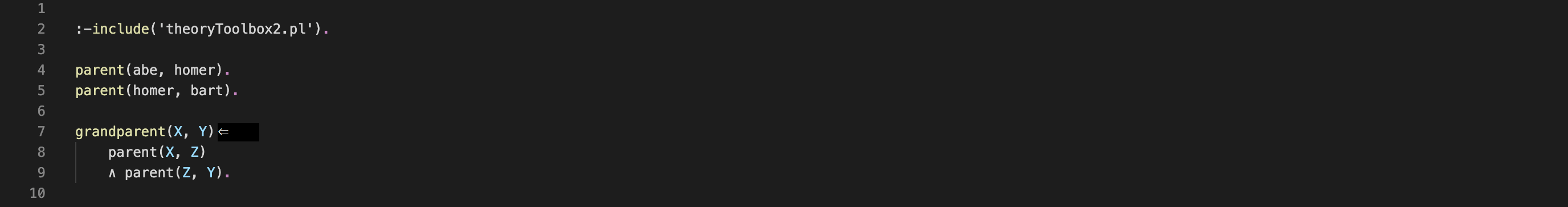
In the antecedent of a clause, atomic formulas and constraints can be combined with conjunction (∧), disjunction (∨) and equality (=). A conjunction A₁ ∧ A₂ ∧ ... ∧ A_n is provable if each A_i is provable (i = 1, 2, ..., n). A disjunction A₁ ∨ A₂ ∨ ... ∨ A_n is provable if at least one A_i is provable (i = 1, 2, ..., n). Equality can be used to impose the restriction that two constants have to be equal (techincally equality is used to indicate unification; more about that later). Ordinary parentheses are used to indicate precedence as usual. Any atom A in the antecedent of a clause can be negated by writing ¬A, which means that A is not provable; i.e. A is not entailed by the program. Note that this is different from saying that A is not the case. That A is not the case has to be indicated explicitly, e.g. with a probability of 0: p(A, 0)., which means that it is provable that A has a probability of zero (A is not the case).

Clauses with a non empty antecedent usually contain variables, and they therefore describe general relations. For example, aunt(A, C) ⇐ sister(A, M) ∧ parent(M, C) means that the aunt relation holds for any A, C and M; i.e. variables are (implicitly) universally quantified. The scope of a variable is the clause in which it appears. This means that same named variables in a clause have to be instantiated with the same constant (between clauses same named variables can be instantiated with different constants). So for example, sister(A, marge) and parent(marge, C) would both have to hold in order for the antecedent sister(A, M) ∧ parent(M, C) to hold (note that M could replaced with marge in both cases).

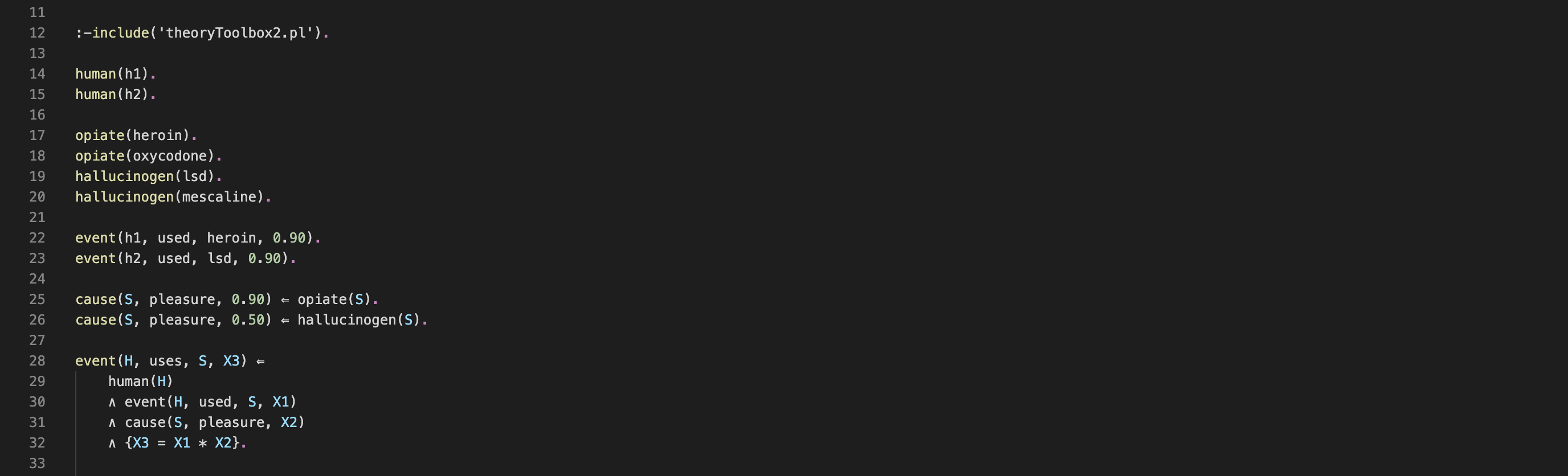
Consider another example that mixes qualitative and quantitative relations, shown in Figure 2. In the example we use an event predicate with a subject, a verb, an object and a probability value. In addition to stating that h1 is a human, that heroin is an opiate and so on, it also says that, among other things, h1 used heroin with a probability of 0.90 and that an opiate causes pleasure with probability 0.90. The last clause has the following meaning. For all H, S, X1, X2, X3, it is provable that H uses S with probability X3 if all of the following conditions hold: H is a human, H used S with probability X1, S causes pleasure with probability X2, X3 is equal to the product between X1 and X2.

Figure 2. A Toy Program that Mixes Qualitative and Quantitative Relations

Before ending this section something needs to be said about the relation between Theory Toolbox 2 and Prolog. Readers who are familiar with Prolog might have noted that our examples do not use standard Prolog syntax (in which comma is used for conjunction and :- for implication). But actually, "under the hood", all code is Prolog: Before running a program, Theory Toolbox 2 uses term_expansion/2 and goal_expansion/2 to replace ∧ with ,, ∨ with ;, ¬ with \+, and ⇐ with :-. So if this is preferred, it is possible to write a theory program in pure Prolog and to use Theory Toolbox 2 on this program. Readers who want to know more about Prolog can check out the excellent introduction Learn Prolog Now by Patrick Blackburn, Johan Bos and Kristina Striegnitz. A more advanced text is Markus Triska's The Power of Prolog.

4. Design Principles for Scientific Theories

With this background, we can now discuss some general design principles for building actual theory programs. The text below contains a brief summary of some of the principles discussed in Rohner and Kjellerstrand (2021) and some additional remarks.

• A scientific theory consists of a set of definite clauses that contain a qualitative and quantitative description of events, relations between events, including any background assumptions on which these relations depend. Every component of a theory a definite clause. Consider the main clauses in the emotion theory. Note, for example, that each emotion is described as an implication, in which the consequent (the probability of the emotion) depends on a set of necessary and sufficient conditions in the antecedent.
• The clauses in a theory can usually be grouped into background clauses and main clauses. Background clauses represent the background assumptions of a theory. Main clauses represent the main relations of a theory. Consider the emotion theory again. The main parts of the theory are the clauses that describe each one of the five emotions; accordingly, these clauses are listed under main clauses. The other clauses, e.g. about what kinds of things people value, which events are congruent with a certain goal, and so on, are background assumptions, so these are listed under background clauses.
• The constructs (concepts) in a theory can be represented by a five argument event atom. Its components are a subject, a verb, an object, a time frame, and a probability value (but any number of additional arguments, such as a place argument, can be added if relevant). By doing so a theory program represents the meaning of constructs, not just their names. Moreover any argument can be a constant, a variable or a function. The emotion theory, for example, contains several such event atoms. Note also that a function is used as the object argument in each emotion clause to distinguish between appraisal and what is appraised. In fear, for example, appraisal is about a future goal incongruent event.
• In addition to the usual symbols of logic, the relations of a theory can be described with a set of equations that relate the probabilities (or other magnitudes) of different events. So in the emotion theory, to take an example, the probability of an emotion depends on the probabilities of different appraisal patterns (see the main clauses of the theory).
• In the clauses of a theory, the domains of all variables should be defined intensionally. This explicitly states the objects that the theory is about, in terms of a set of necessary and sufficient conditions. For example, in the main clauses of the emotion theory, H1, H2, E and G and so on, are defined to be humans, events, and goals, respectively.
• Finding out how the probabilities of different events are functionally related depends on induction from empirical observations. Empirical observations, in turn, depend on having a preliminary theory that defines what should be observed when and where. Such a preliminary theory can be encoded in a logic theory program in which any probability equations are left undefined (these are defined after the functional relations between probabilities become known through empirical observation). An example can be found here

5. Advantages of Logic Programming

This section briefly describes some of the advantages of logic programming. An in depth discussion of these advantages can be found in Rohner and Kjellerstrand (2021).

• Validity. When a theory is represented in a logic program it is possible to use resolution to derive valid conclusions from it. A valid conclusion is a conclusion that has to be true if the information in the program is true. Schematically, M ∧ B ⊨ C, where M is the set of main clauses, B the set of background clauses, and C the conclusion. So when a theory is a good one one, it can be used to generate accurate predictions and explanations. This aspect is relevant whenever a scientific theory is used to generate new knowledge or in an applied setting.
• Explicit Background Assumptions. Because first order logic can represent almost any kind of relation, it is possible to build a detailed formalization of the background assumptions in a theory. Any prediction C from a theory is then entailed by its main clauses M and its background clauses B: M ∧ B ⊨ C. So if states of affairs are at odds with C, the blame has to fall on either M or B, or both M and B. When (informally) inferring empirical predictions from a natural language representation, in contrast, there is a higher risk that we unwittingly presuppose one or more Bs that were never in the theory. So a test of such a prediction becomes ambiguous: If a B wasn't in the theory, an empirical test that assumed this B is not a test of the theory.
• A Representation of both the Qualitative and Quantitative Parts of a Theory. By using predicates, such as the event predicate, in addition to the usual symbols of logic, is is possible to capture important qualitative information that is usually expressed in natural language. And the possibility to nest an arbitrary number of functions in an atomic formula, increases this expressive power even further. Such qualitative information can be combined with any number of equations that relate probabilities or other quantities. Note also that when the semantic content of events is decomposed into subject, verb, object, time and value arguments, is is possible to represent some important relations between the intra event components of different events in a clause.
• Universal Statements About Well Defined Domains. Scientific theories consist of a set of universal statements that describe relations between all events of a certain kind; i.e. they are nomothetic descriptions (Popper, 1972). A powerful feature of first order logic is that is is possible to explicitly say that a certain relation holds for all objects in one or more sets and to provide detailed definitions of these sets. This is achieved by using variables and by writing any domain definitions in the antecedent of a clause.
• Modularity. Another powerful feature of logic programs is that they are modular representations, meaning that: (1) It is possible to add any number of components to a theory without modifying the components that already exist in the theory. (2) Adding components to a theory will usually make the theory entail more information than just the information contained in the added components.
• Rational Theory Evaluation. Because theory programs are formal representations, it is possible to hand them to algorithms that perform basic sanity checks, already before empirical testing. For example, Theory Toolbox 2 has predicates that ckeck whether a theory is internally coherent, how general it is, and if it subsumes one or more other theories.
• Collaboration. Theory programs can be uploaded to an online software hosting and version control platform such as GitHub. This has the following advantages: (1) Members of a reasearch team can suggest and make changes to the theory online; (2) It is easy to keep track of any changes to the theory; (3) members of the team instantly have the latest version of the theory available on their computer (the local version of the theory is synchronized to the online one); (4) members of the team can instantly run queries on the latest version of the theory (e.g. using Theory Toolbox 2).
• Plan Representative Empirical Studies. Finding out how the probabilities of different events are functionally related depends on induction from a set of empirical observations, e.g. with logistic regression. And empirical studies in turn depend on having a preliminary theory that defines relevant domains. Theory Toolbox 2 can generate a plan for an empirical study that is representative with respect to a theory (e.g. if a theory is about arithmetic performance, a plan for an empirical study should randomly sample from the universe of all relevant integers and all relevant operations on these integers).

6. Using Theory Toolbox 2

6.1. Introduction

Theory Toolbox 2 is a collection of Prolog predicates for using, evaluating and building scientific theories. Here is a brief description of what each predicate does. Details and usage examples for each predicate are in sections 6.4. to 6.12.

Deducing predictions

provable/3: Finds any conclusions that are entailed by a theory.

Generating explanations

prove/3: Finds proofs for any conclusions that are entailed by a theory.

maxValue/4 and minValue/4: Find proofs such that the value of a numerical variable is maximized/minimized.

Rational theory evaluation

incoherence/7: Checks whether a theory is internally coherent (not self contradictory).

falsifiability/3: Counts the number of predictions that are entailed by a theory.

subsumes/5: Checks whether one theory subsumes another theory; i.e. it makes all the predictions that the other theory makes and more.

Planning empirical studies that are representative of a theory

allClauses/3: Finds all clauses with a certain consequent that are entailed by a theory.

generateRandomObjects/4: Generates random objects of a certain kind.

sampleClauses/5: Yields a simple random sample or a stratified random sample of all clauses that are entailed by a theory.

NOTE: Theory Toolbox 2 is experimental software that is in continuous development and provided as-is; so you may encounter various bugs (see the license for more info). In case you have any questions, feedback or find any problems, please post an issue.

6.2. Proof Search

A common feature of the predicates in Theory Toolbox 2 is that they all, in some way or another, deal with the conclusions that are entailed by a theory program. The search for such conclusions starts with a query goal, an atomic formula which may or may not contain variables. If the goal only contains constants, the output is true (or false), meaning that it is true (or false) that this goal is entailed by the theory program. If the goal contains one or more variables, all the variable instantiations that are entailed by the program are shown. As an example, suppose the query goal is grandparent(abe, bart). , which in relation to Figure 1, means "does the program entail that the grandparent trelation holds between Abe and Bart?". In this case the answer would be true. The query goal grandparent(abe, X), instead means "for what Xs does the relation in which Abe is the grandparent hold according to the program?". In this case we get any constants for which the goal holds (is provable); i.e. X = bart.

So in what cases exactly is a goal provable? In other words, in what cases does a theory program entail a goal? Before explaining this, a basic understanding of unification is necessary, because unification is an essential part of proof search. Unification is about determining if two formulas match or not; syntactically unification is indicated by the equality sign =. Two formulas unify in the following important conditions:

1. Two constants unify if they are the same
2. A variable unifies with any kind of term and is instantiated to that term
3. Two atomic formulas, or functions, unify if all of these conditions hold:
1. They have the same name
2. They have the same number of arguments
3. All of their arguments unify
4. Their variables can be instantiated consistently

So according to rule 1, bart = bart, 1 = 1, and 3.14 = 3.14. According to rule 2, X = bart and Y = event(john, like, mary). And according to rule 3 event(H1, represent, Representation) = event(H1, represent, event(H1, like, H2)), because both atoms have the same name (event), the same number of arguments (3), because H1 = H1, because represent = represent, and because Representation = event(H1, like, H2). But, according to rule 3d, foo(X, X) = foo(2, 3) fails because X is first instantiated to 2 and then 2 does not unify with 3.

And now we finally get to the conditions for when a goal is provable (without going into technical details). A goal is provable in each one of the following cases:

1. The goal is true, e.g. as in {4 = 2 + 2}, or {X = 2 + 3, X > 1}.
2. The goal unifies with the consequent of a clause that has an empty antecedent (when the antecedent is empty the consequent holds unconditionally).
3. The goal unifies with the consequent of a clause whose antecedent is provable (per modus ponens, the consequent holds if the antecedent holds).
4. The goal unifies with a term in INPUT

But what does INPUT mean? More about that in the next section.

6.3. The INPUT argument

All of the predicates in Theory Toolbox 2 have an argument called INPUT. INPUT is used to temporarily assert anything that is considered provable in addition to the information in a theory program. Because theories should only contain general statements, they are not supposed to be filled will all the particular instances to which they may be applied. For example, a theory about kinship, should not contain clauses about Homer being the parent of Bart and so on (see Figure 1). Information about particular instances should be provided in INPUT instead. Per se, the theory should only contain general statements like grandparent(G, C) ⇐ parent(G, P) ∧ parent(P, C). . Syntactically, INPUT is a Prolog list, i.e. a comma delimited list of atomic formulas in square brackets. So by writing, for example, INPUT = [parent(jaqueline, marge), parent(marge, lisa)], we declare that these goals are provable in addition to the information in a theory program.

Note that all theory examples contain a commented section INPUT. This is a declaration of what atoms that have to be provided in INPUT in order for all the consequents of a theory to be provable. Providing such a section is not necessary but it is a favour to any third parties that wish to use a theory. Practical examples in which INPUT is used follow below.

6.4. provable/3

provable(GOAL, INPUT, RESULT) queries if GOAL is provable given INPUT and unifies the result with RESULT. In case GOAL only contains constans, the output is true or false. In case GOAL contains any variables, RESULT is unified with any variable instantiations in GOAL that are entailed by the program.

• GOAL should be an atomic formula with constants, variables or functions as arguments.
• INPUT should be a list of zero or more atomic formulas.

showProvable(RESULT) prints the result obtained from provable(GOAL, INPUT, RESULT) to the console.

Figure 3 shows two queries with provable/3 and the associated output predicate showProvable/1. The underscores in the goal are anonymous variables. An anonymous variable unifies with anything, like an ordinary variable (written with an initial capital letter). Using an anonymous variable for an argument in the goal is equivalent to saying "Whatever the theory entails for this argument and predicate.". Note, for example, that aunt(selma, lisa) holds because the information that leads up to this conclusion is a combination of the clauses in the program and the information in INPUT (see the discussion in the previous section).

Figure 3. provable/3 Used on a Toy Example

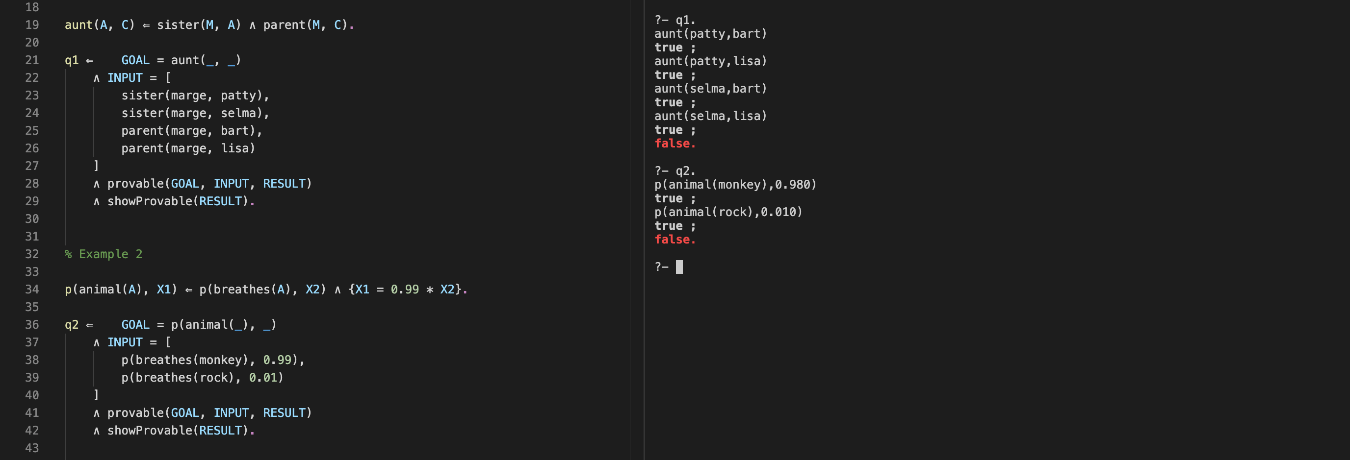
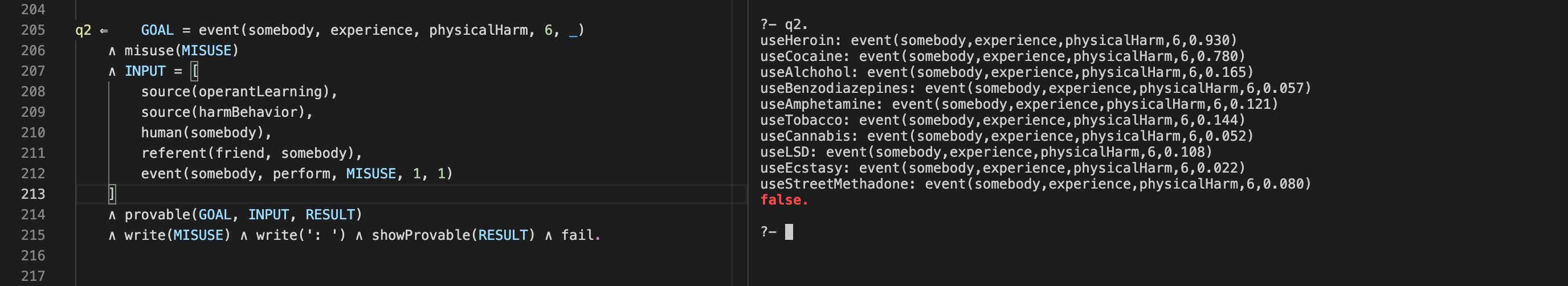
Figure 4 shows a query on the substance misuse example. The query goal means "the probability that somebody experiences harm at time 6" (value was the last argument in event). The line misuse(MISUSE) unifies MISUSE with any misuse behavior in the theory (e.g. useHeroin). This variable is then used in INPUT to assume that somebody performs that behavior in time frame 1 with probability 1. After the call to provable/3, showProvable/1 is used to print a solution to the console; write and fail are built-in Prolog predicates that print to the console and show all solutions, respectively.

The output shows different probabilities of experiencing physical harm. Note that some substances cause more harm at time 6 even if they have lower harm values in the background clauses of the theory; this is because some substances cause more pleasure than others (increasing the likelihood of misuse, and therefore harm).

Figure 4. provable/3 Used on the Substance Misuse Example

Examples in which provable/3 is used are:

• tutorialExamples.pl
• substanceMisuseExampleState.pl
• collinsQuillianExample.pl
• planningExample.pl
• substanceMisuseExample.pl
• phobiaExample.pl

6.5. prove/3

prove(GOAL, INPUT, RESULT) finds a proof for GOAL given INPUT and unifies the result with RESULT. In case GOAL is not provable, the result is false.

• GOAL should be an atomic formula with constants, variables or functions as arguments.
• INPUT should be a list of zero or more atomic formulas.

showProof(RESULT, OPTION) prints the proof obtained from prove(GOAL, INPUT, RESULT) to the console.

• OPTION should be one of the following: monochrome, color, lanes.

Note: In case the system of equations in a theory doesn't have a unique solution, prove/3 returns a symbolic solution with all the computations that lead up to the goal.

Figure 5 shows a query with prove/3 and its output predicate showProof/2. In the query note that, as in previous examples, underscores (anonymous variables) are used to get "whatever the theory entails for this argument and predicate", and that the particular objects to which the theory is applied are put in INPUT. The output shows all the steps that lead up to the conclusion (at the top). Here, the antecedents for a given consequent are shown just below the consequent, indented to the right. Goals from the same clause are shown in the same color and level of indentation.

Figure 5. prove/3 Used on a Toy Example

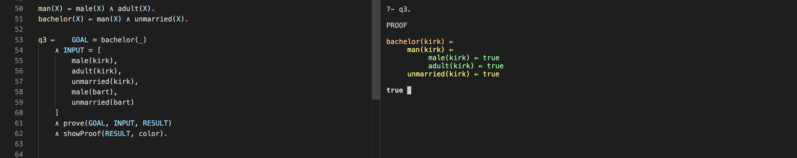
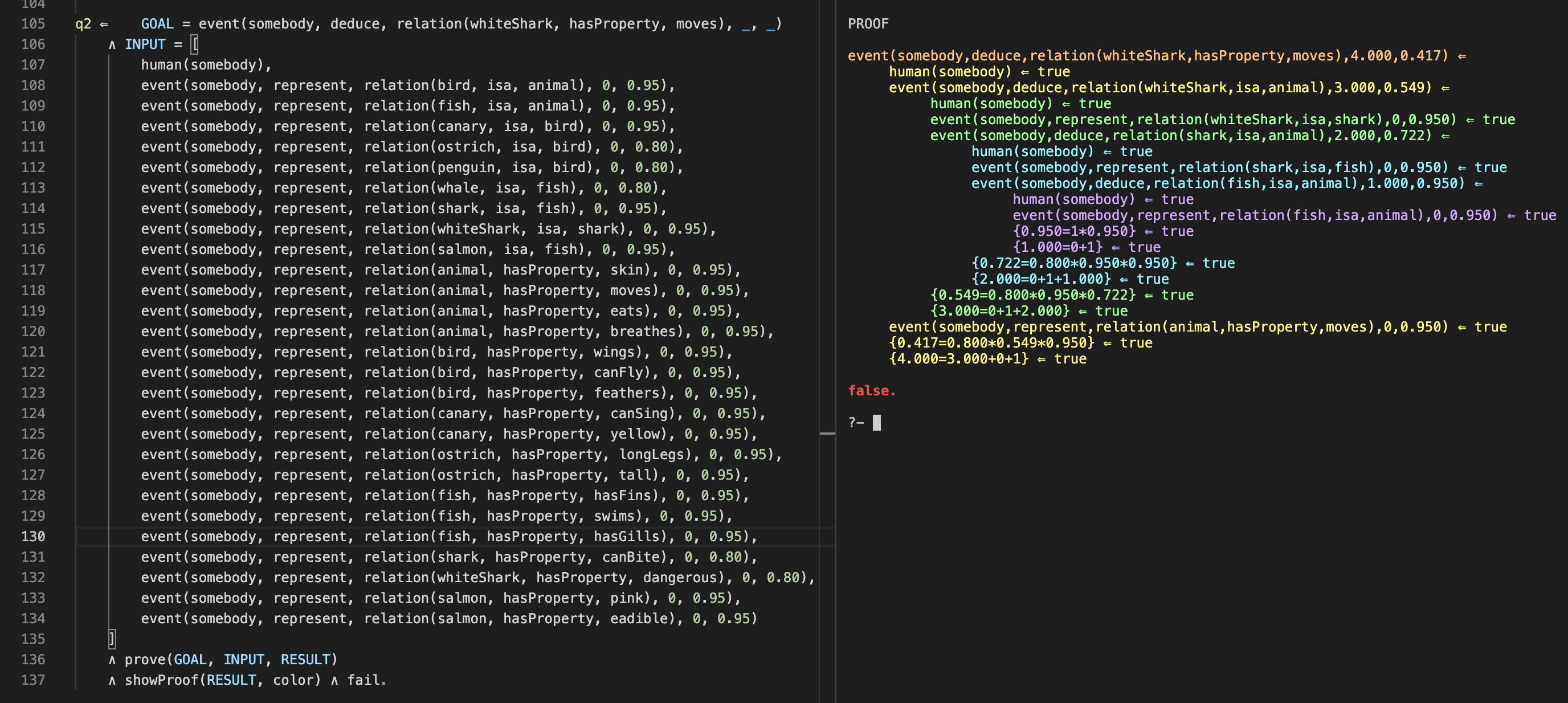
Figure 6 shows a query with prove/3 on the collinsQuillian example. The goal means "somebody can deduce that a white shark moves in some time frame and with some probability"; by using anonymous variables (underscores) for these arguments we leave it up to prove to find whatever constants the theory entails for this relation.

Figure 6. prove/3 Used on the Collins and Quillian Example

Examples in which prove/3 is used are:

• tutorialExamples.pl
• collinsQuillianExample.pl
• substanceMisuseExample.pl
• substanceMisuseExampleState.pl
• planningExample.pl
• naturalSelectionExample.pl
• inferenceWithUnknownInformation.pl

6.6. maxValue/4 and minValue/4

maxValue(X, GOAL, INPUT, RESULT) finds a proof for GOAL given INPUT, such that the value X in GOAL is as high as possible; the result is unified with RESULT. In case GOAL is not provable the output is false.

• GOAL should be an atomic formula with constants, variables or functions as arguments, where the argument X is a numerical variable.
• INPUT should be a list of zero or more atomic formulas.

Note: Exogenous numerical variables, i.e. variables that do not appear as dependens in any theory equation, should be unified with a set of numerical constants in the theory or in INPUT.

showMaxValue(RESULT, OPTION) prints the results obtained from maxValue(X, GOAL, INPUT, RESULT) to the console.

• OPTION should be one of the following: monochrome, color, lanes.

minValue(X, GOAL, INPUT, RESULT) and showMinValue(RESULT, OPTION) have the same functionality, except that they find an show a proof such that the numerical argument X is as low as possible.

Figure 7 shows maxValue/4 applied to a toy example. In the theory (to the left) note that we assign a set of alternative values to exogenous numerical variables (numerical variables that do not appear as dependents in any theory equation). This means that the numerical variable associated with profit (X1), for example, can take on all values that result from using 0, 5 and 10 in the theory equations. In the query, the goal contains the variable X. Note that X also appears in maxValue(X, GOAL, INPUT, RESULT) further down. This tells maxValue/4 that it is the value of X we want to maximize.

The output shows a proof for the goal, which is such that the X variable in the goal is as high as possible. Note that the proof shows all the constants and numerical computations that lead up to this conclusion.

Figure 7. maxValue/4 Used on a Toy Example

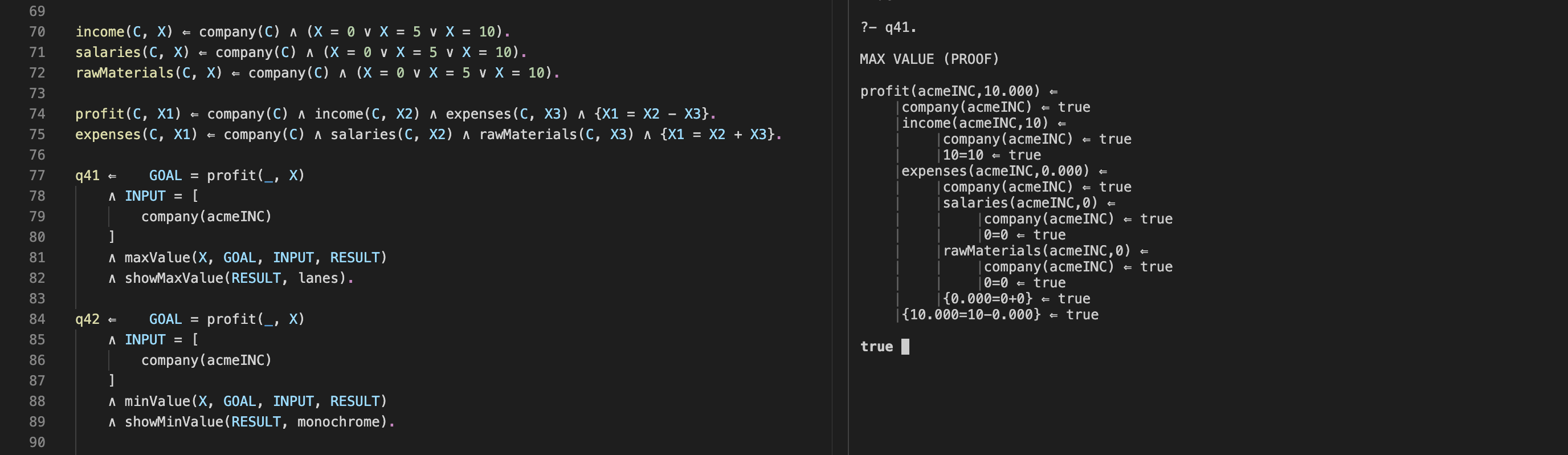
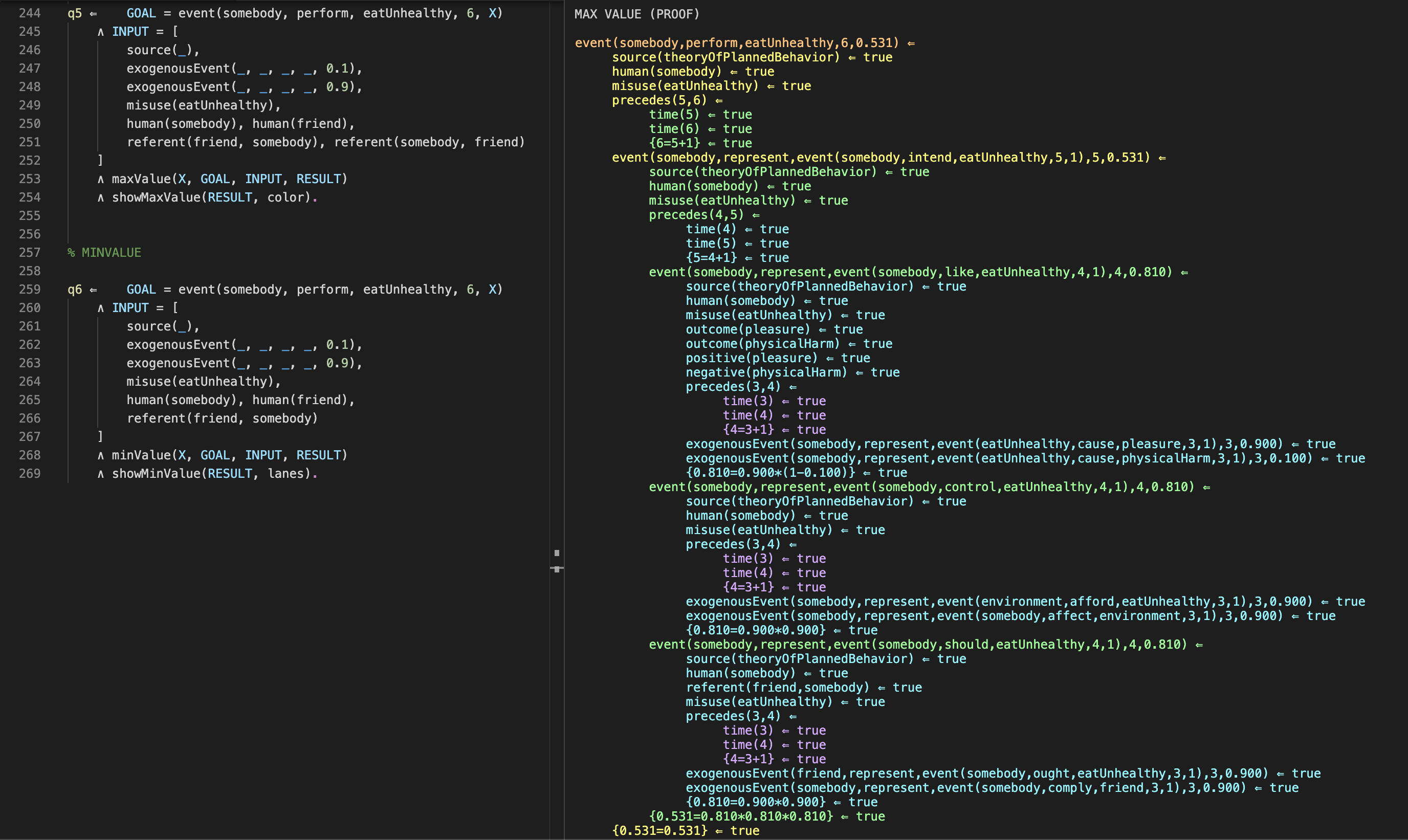
Figure 8 shows an example in which maxValue/4 is applied to substanceMisuseExample.pl. The goal corresponds to "somebody eats unhealthy at time 6 with probability X". Finding a proof that maximizes the value of X is relevant in this case, because it contains an explanation for a problem (why the probability of eating unhealthy is high). INPUT then contains a number of things. First, source(_) assumes that any source holds (an anonymous variable unifies with anything, in this case e.g. theoryOfPlannedBehavior, operantLearning and so on, see the theory). Secondly, exogenousEvent(_, _, _, _, 0.1) and exogenousEvent(_, _, _, _, 0.9) assume that any exogenous event holds with probability 0.1 or 0.9. The reason for assigning values in these predicates is that, in the theory, their equations have independent variables that are exogenous (variables that do not appear as dependents in any theory equation). Third, misuse(eatUnhealthy) allows the theory to be applied to this behavior as well (eating unhealthy was not defined as a misuse behavior in the background clauses). Finally, INPUT contains the other prerequisites defined in the INPUT section of the theory.

The output contains a proof which is such that values of exogenous variables maximize the numerical argument X in the goal. Note how these values then propagate in the systems of equations that lead up to X. For example, we can see that some of the explanations for eating unhealthy are that a person believes that eating unhealthy causes pleasure and believes that eating unhealthy does not cause physical harm.

Figure 8. maxValue/4 used on the Substance Misuse Example

Examples in which maxValue/4 and minValue/4 are used are:

• tutorialExamples.pl
• emotionExample.pl
• substanceMisuseExample.pl
• sourceMonitoringExample.pl
• neuropharmacologyExample.pl

6.7. incoherence/7

incoherence(GOAL1, GOAL2, INPUT, THRESHOLD, X1, X2, RESULT) checks if GOAL1 and GOAL2 differ with respect to their numerical values X1 and X2, more than THRESHOLD given INPUT. The result is unified with RESULT. In case there is no incoherence, the output is false.

• GOAL1 and GOAL2 should be atomic formulas that each contain a numerical variable; for example X1 and X2, respectively.
• INPUT should be a list of zero or more atomic formulas.
• THRESHOLD should be a number (integer or real).
• X1 and X2 are the numerical variables in GOAL1 and GOAL2.

showIncoherence(RESULT, OPTION) prints the results obtained from incoherence(INPUT, GOAL1, GOAL2, THRESHOLD, X1, X2, RESULT) to the console.

• OPTION should be one of the following: monochrome, color, lanes.

Figure 9 shows a toy example with incoherence/7. Note that GOAL1 and GOAL2 have the same variables for the first two arguments (A and B), but that the last value arguments are X1 and X2. In this way it is possible to check whether a theory entails that two goals that have the same meaning (represented by A and B) have different probabilities (i.e. an incoherence). Remember that same named variables in a clause have to hold the same constants.

Figure 9. incoherence/7 Used on a Toy Example

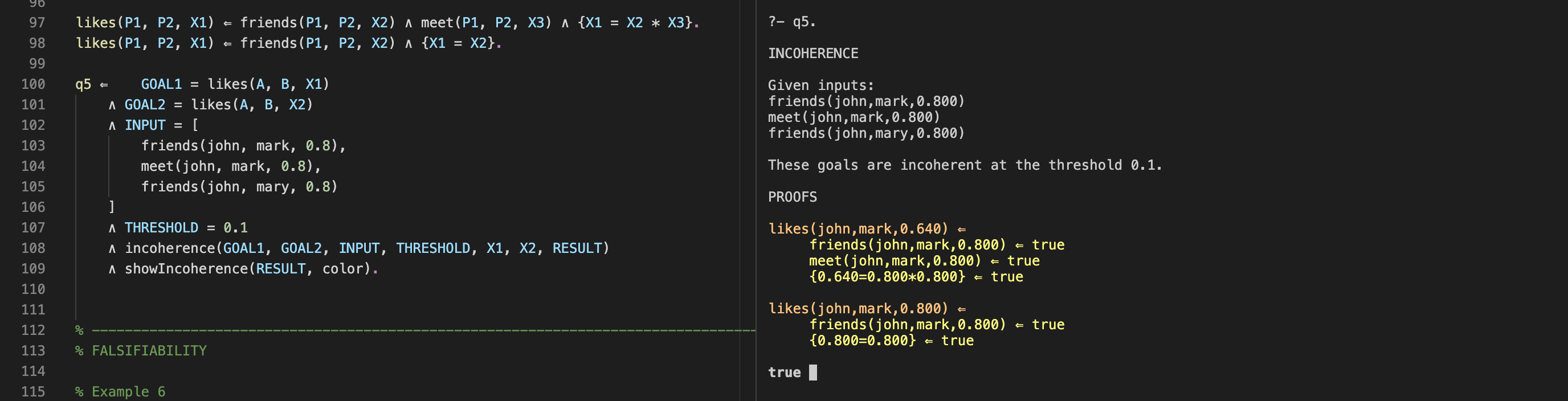
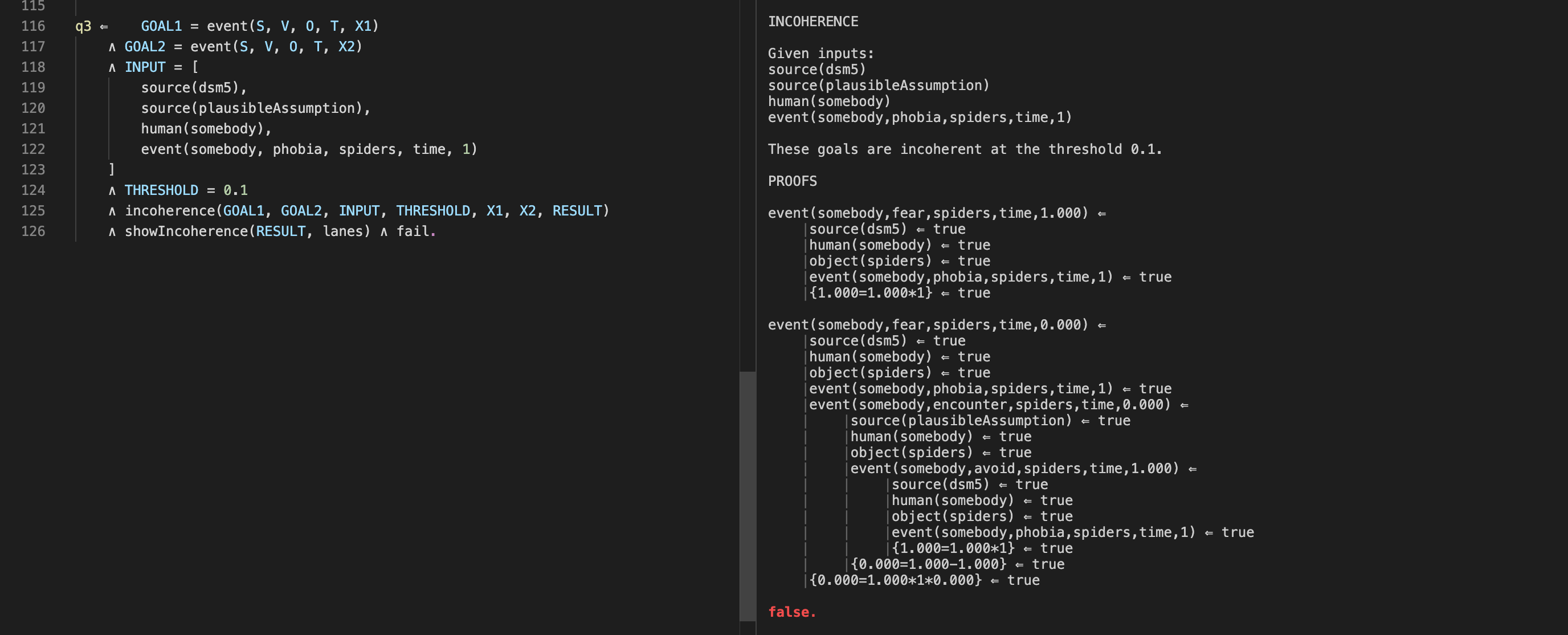
Figure 10 shows incoherence/7 applied to phobiaExample.pl. Note that in GOAL1 and GOAL2 the first four arguments contain the same variables; this means that both goals have to have the same subject, verb, object and time frame (given that same named variables in a clause have to hold the same constants). The output shows that there is an incoherence in the theory: It entails that the probabilities of fear are different, even if the input is the same. The proof shows why this happens. Note that the clause about the negative relation between avoiding an object and encountering an object is involved.

Figure 10. incoherence/7 Used on the Phobia Example

Examples in which incoherence/7 is used are:

• tutorialExamples.pl
• phobiaExample.pl

6.8. falsifiability/3

falsifiability(GOAL, INPUT, RESULT) counts the number of unique predictions with respect to GOAL given INPUT and unifies the result with RESULT.

• GOAL should be an atomic formula with constants, variables or functions as arguments.
• INPUT should be a list of zero or more atomic formulas.

showFalsifiability(RESULT) prints the results of falsifiability(GOAL, INPUT, RESULT) to the console.

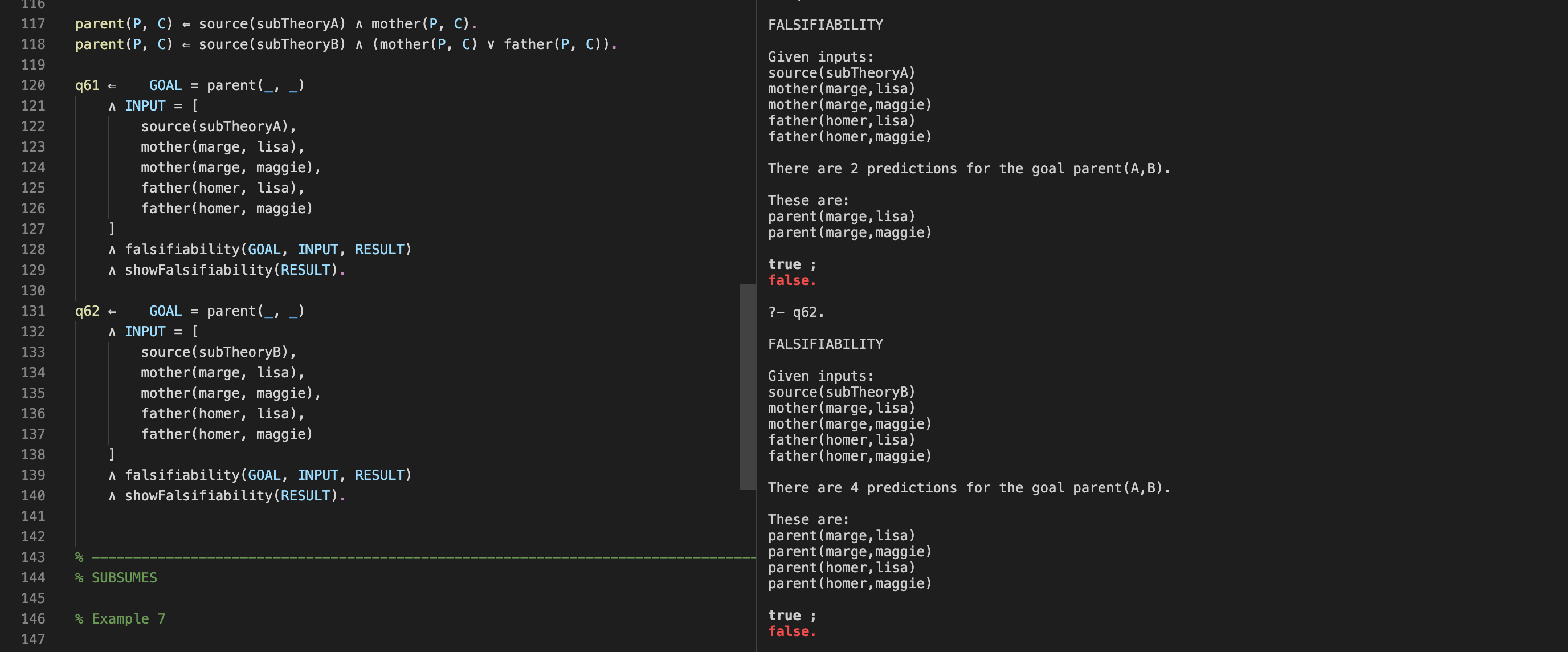
Consider Figure 11 which shows a toy example involving falsifiability/3. In the example there are two subtheories: subTheoryA and subTheoryB. The second one is more general because a parent is defined as either a mother or a father. Note that in q61 and q62 the information in INPUT is the same, except that in the first case subTheoryA holds and in the second case subTheoryB holds. The output shows that subTheoryB is more falsifiable because it makes more predictions; i.e. it is a more general theory.

Figure 11. falsifiability/3 Used on a Toy Example

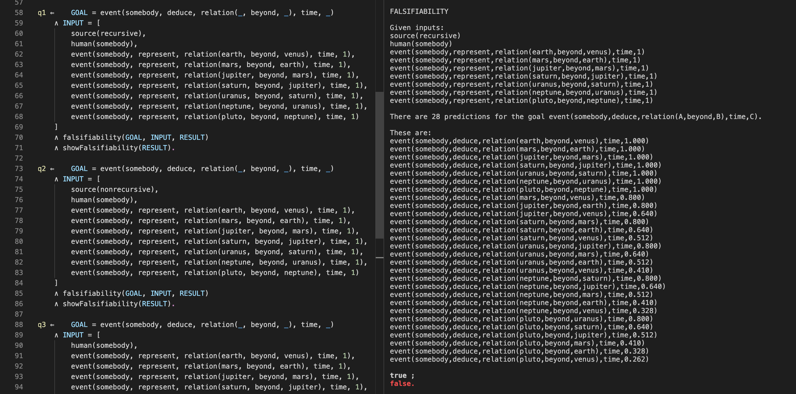
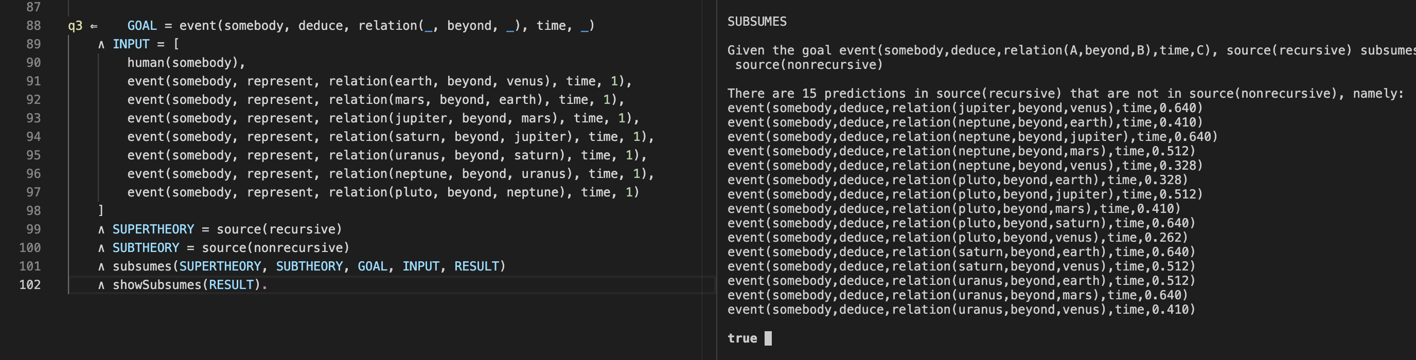
A realistic example is shown in Figure 12, which is based on distanceExample.pl. The goal means "somebody can deduce that some object is beyond some other object at some time with some probability". This theory has a recursive part and a non recursive part. In INPUT the recursive part is assumed to hold. The output shows that the theory generates 28 predictions. Replacing source(recursive) with source(nonrecursive) in INPUT only generates 13 predictions (not shown). The recursive theory is therefore more falsifiable and general.

Figure 12. falsifiability/3 Used on the Distance Example

Examples in which falsifiability/3 is used are:

• tutorialExamples.pl
• distanceExample.pl

6.9. subsumes/5

subsumes(SUPERTHEORY, SUBTHEORY, GOAL, INPUT, RESULT) checks if SUPERTHEORY subsumes SUBTHEORY with respect to GOAL given INPUT and unifies the result with RESULT.

• GOAL should be an atomic formula with constants, variables or functions as arguments.
• SUPERTHEORY and SUBTHEORY should be atomic formulas.
• INPUT should be a list of zero or more atomic formulas.

Note: Clauses that belong to SUPERTHEORY should have SUPERTHEORY in their antecedent; clauses that belong to SUBTHEORY should have SUBTHEORY in their antecedent. INPUT should not contain SUPERTHEORY and SUBTHEORY.

showSubsumes(RESULT) prints the results from subsumes(SUPERTHEORY, SUBTHEORY, GOAL, INPUT, RESULT) to the console.

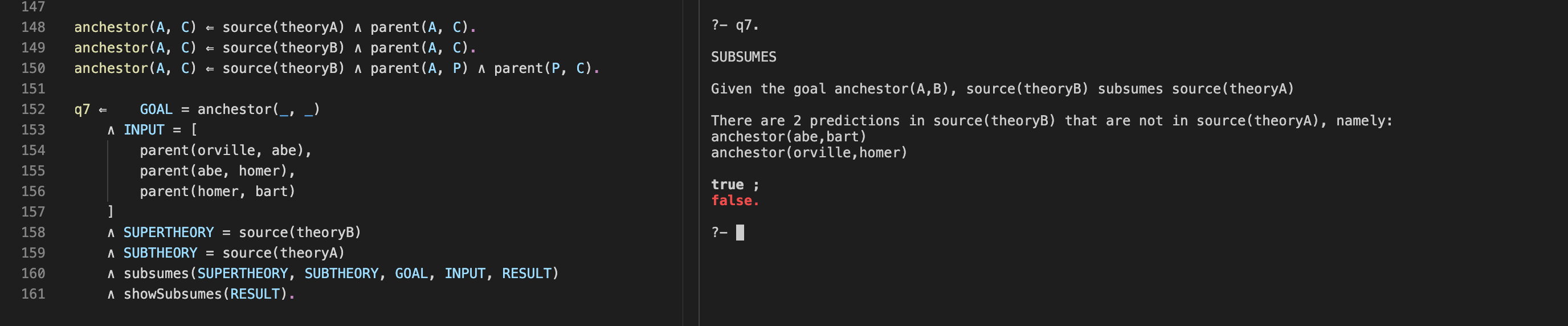
Figure 13 shows a toy example in which subsumes/5 is used. The goal means "the objects for which the anchestor relation holds". Theory B subsumes theory A because in theory B, an ancestor is either somebody's parent or somebody's grandparent.

Figure 13. subsumes/5 Used on a Toy Example

A realistic example is shown in Figure 14, which is based on distanceExample.pl. The goal corresponds to "somebody can deduce that some object is beyond some other object at some time with some probability". The clauses of this theory either contain an atom source(recursive) or source(nonrecursive). In the query these are used as arguments to subsumes/5 to find out if the recursive theory subsumes the non recursive one. As shown in the output, the recursive theory indeed subsumes the non recursive one; i.e. all the predictions in the non recursive theory also exist in the recursive one.

Figure 14. subsumes/5 Used on the Distance Example

Examples in which subsumes/5 is used are:

• tutorialExamples.pl
• distanceExample.pl

6.10. allClauses/3

allClauses(GOAL, INPUT, RESULT) generates all clauses that have the consequent GOAL and that hold given INPUT; results are unified with RESULT.

• GOAL should be an atomic formula with constants, variables or functions as arguments.
• INPUT should be a list of zero or more atomic formulas.

showAllClauses(RESULT) prints the results obtained from allClauses(GOAL, INPUT, RESULT).

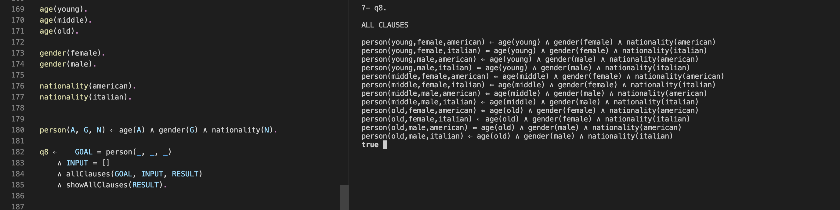
Figure 15 shows a toy example. The goal denotes a person with three properties; according to the theory these are age, gender and nationality. The output (in the right part of Figure 15) shows all clauses that hold for this goal.

Figure 15. allClauses/3 Used on a Toy Example

Examples in which allClauses/3 is used are:

• tutorialExamples.pl

6.11. generateRandomObjects/4

generateRandomObjects(FRAMESIZE, SAMPLESIZE, PREDICATENAME, RESULT) generates a list RESULT of length SAMPLESIZE containing atomic formulas with predicate name PREDICATENAME and random integers in the range 1 to FRAMESIZE as the argument.

• FRAMESIZE and SAMPLESIZE should be integers such that FRAMESIZE > SAMPLESIZE.
• PREDICATENAME should be a textual constant.

An example with generateRandomObjects/4 is shown in Figure 16. Five random objects are sampled from all objects in the range 1 - 1000.

Figure 16. generateRandomObjects/4 Used on a Toy Example

Examples in which generateRandomObjects/3 is used are:

• tutorialExamples.pl

6.12. sampleClauses/5

sampleClauses(GOAL, INPUT, N, STRATIFY, RESULT) randomly samples N clauses from each stratum defined in STRATIFY, where all strata have the consequent GOAL and hold given INPUT. Unify the result with RESULT.

• GOAL should be an atomic formula with constants, variables or functions as arguments
• INPUT should be a list of atomic formulas
• N should be an integer
• STRATIFY should be an empty list or a list of atomic formulas

Note: If STRATIFY is an empty list, the result is a simple random sample of size N (without stratification). Otherwise, strata are all combinations of all groundings of the atomic formulas in STRATIFY. E.g. if STRATIFY = [p(_), q(_)], and the groundings of p(_) and q(_) are p(a), p(b), q(c) and q(d), strata are p(a) ∧ q(c), p(a) ∧ q(d), p(b) ∧ q(c) and p(b) ∧ q(d). A maximum of 4 stratification predicates can be used in STRATIFY.

showSampleClauses(RESULT) prints the results from sampleClauses(GOAL, INPUT, N, STRATIFY, RESULT) to the console.

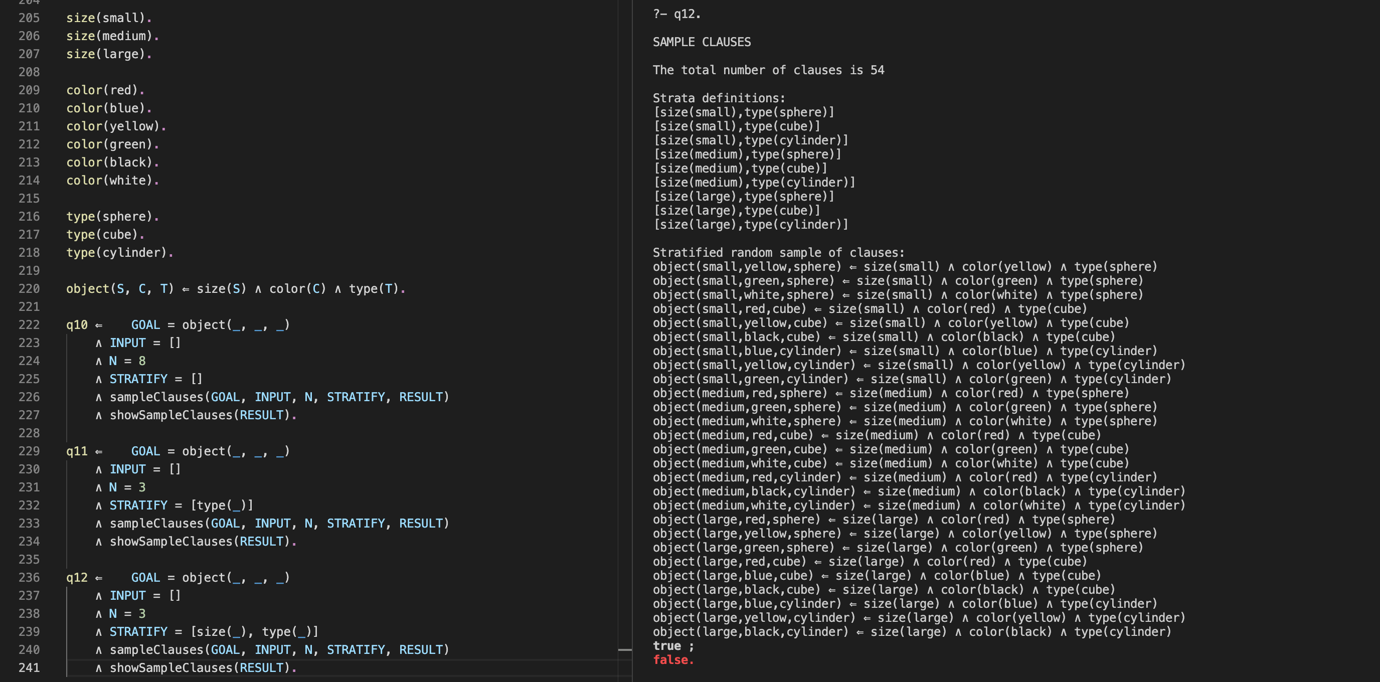
Figure 17 shows a toy example involving sampleClauses/5. In query 12, the goal denotes an object with three properties. We wish to draw a sample of three clauses from each stratum. STRATIFY = [size(_), type(_)] indicates that we want a random sample from each stratum that results by combining all groundings of size(_) and type(_). In the output, in the right part of Figure 17, we are given all strata definitions, followed by a stratified random sample of clauses. Note that three clauses are randomly sampled from each stratum (such that all strata are represented).

Figure 17. sampleClauses/5 Used on a Toy Example

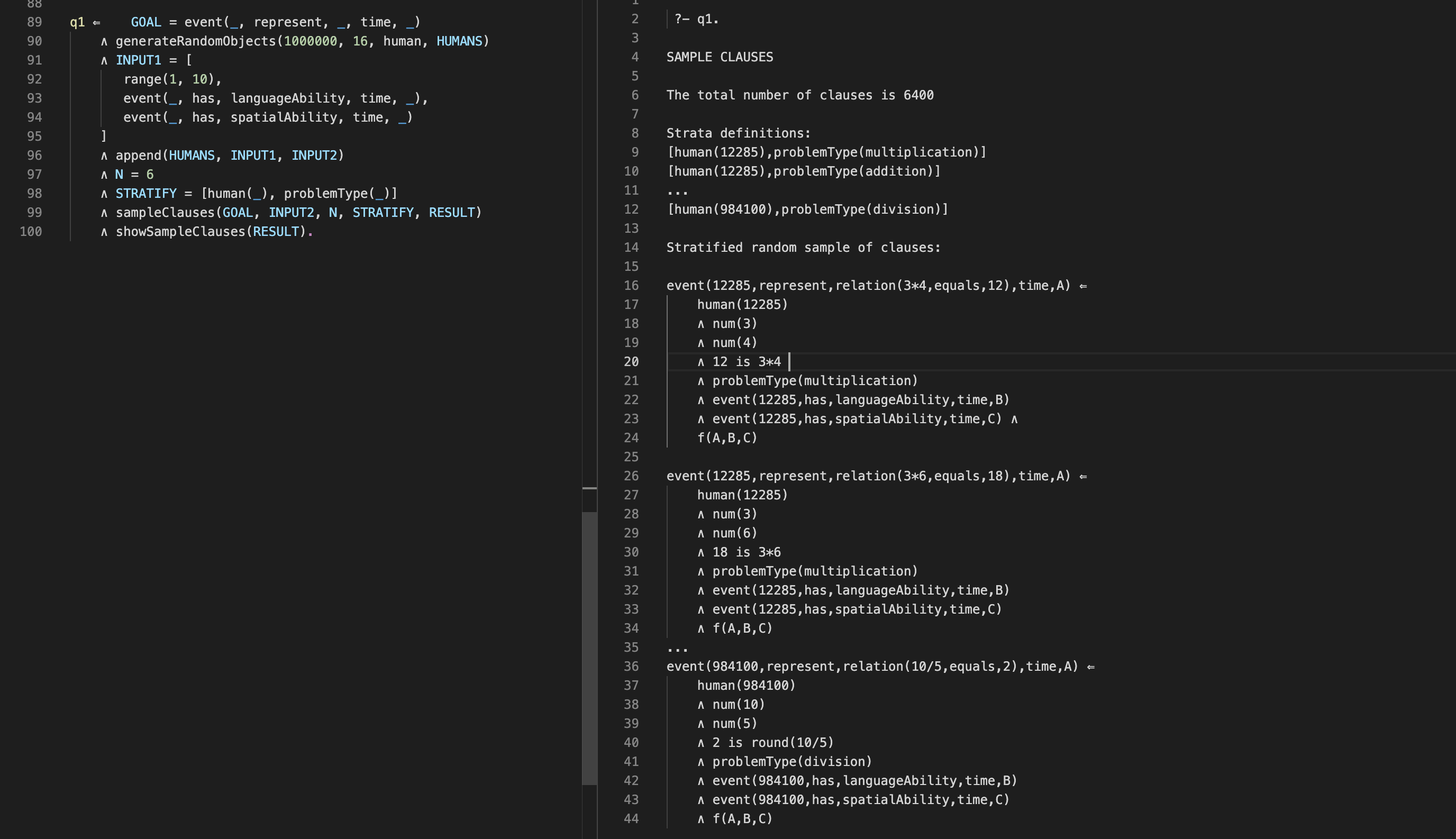
A realistic example involving sampleClauses/5 and generateRandomObjects/4 is shown in Figure 18. It is based on arithmeticExample.pl. The goal denotes whether a person can correctly represent the solution to a certain arithmetic problem (addition, subtraction, multiplication or division as shown in the theory). We then use generateRandomObjects/4 to create a random sample of 16 humans from a population of 1000000. INPUT1 then defines the atomic formulas that are required according to the input section in the theory. Next, INPUT1 is appended to the list of humans, resulting in INPUT2. We want a random sample of 6 clauses from each stratum defined by STRATIFY = [human(_), problemType(_)]; i.e. for each human and for each problem type we want 6 randomly chosen clauses.

The output is shown in the right part of Figure 18. Only a subset of strata definitions and sampled clauses are shown for space reasons. By using sampleClauses/5 and generateRandomObjects/4 it is possible to obtain a representative sample of the population that consists of combinations of 1000000 humans and 400 arithmetic problems (four operations, ten integers, two integers in each operation).

Figure 18. sampleClauses/5 Used on arithmeticExample.pl

Examples in which sampleClauses/5 is used are:

• tutorialExamples.pl
• arithmeticExample.pl

References

• Bratko, I. (2001). Prolog programming for artificial intelligence. Pearson education.
• Popper, K. R. (1972). The logic of scientific discovery. Hutchinson.
• Rohner, J. C. & Kjellerstrand, H. (2021). Using logic programming for theory representation and inference. New Ideas in Psychology, 6, 100838.
• Wielemaker, J., Schrijvers, T., Triska, M., & Lager, T. (2010). Swi-prolog. arXiv preprint arXiv:1011.5332.
• Wielemaker, J., Lager, T., & Riguzzi, F. (2015). SWISH: SWI-Prolog for sharing. arXiv preprint arXiv:1511.00915.

This project would not have been possible without the kind help of several people. On the SWI Prolog forum I want to thank Alan B, Anne O, Carlo C, David T, Eric T, Fabrizzio R, Jan W, j4n_bur53, Paul B, Paulo M and Peter L. On StackOverflow i want to thank Daniel L, @false, @Guy Coder, @lurker, @Mostowski Collapse, @repeat and @mat. At my uni I want to thank Martin B and Erik J O. And a big thanks goes to Håkan K for helping me solve some tricky problems and giving me hands on advice!

The meta-interpreters in Theory Toolbox have been inspired by Sterling and Shapiro's The Art of Prolog and Markus Triska's The Power of Prolog.

All of the algorithms in Theory Toolbox 2 are written in SWI Prolog, a fantastic and free Prolog system.